Plotting in MATLAB
plotmodel
plotmodel takes the model md as first argument and then an even number of options (as in the function setelementstype, or solve). To plot a given field, use the option 'data' followed by the field one wants to plot. For the thickness:
>> plotmodel(md, 'data', md.geometry.thickness)
You can plot several fields at the same time but you have to add the argument 'data' before each field you want to plot:
>> plotmodel(md, 'data', md.geometry.thickness, 'data', 'mesh', 'data', [1:md.mesh.numberofelements])
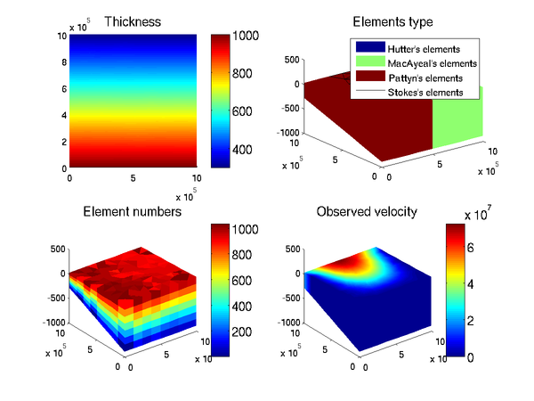
This can work for any field of length md.mesh.numberofelements or md.mesh.numberofvertices.
Options
Options in plotmodel come as pairs: the option name must be followed by its value. For example, if one wants to remove the color bar, the option name is 'colorbar' and the value 0:
>> plotmodel(md, 'data', md.initialization.vel, 'colorbar', 0)
any options (except 'data') can be followed by '#<i>' where <i> is the subplot number, or '#all' if applied to all plots. For example:
>> plotmodel(md, 'data', md.initialization.vel, 'data', 'mesh', 'view#2', 3, 'colorbar#all', 'on', 'axis#1', 'off equal')
axis
Same as standard axis MATLAB option:
>> plotmodel(md, 'data', md.vel, 'axis', 'tight')
view
Same as standard view MATLAB option:
>> plotmodel(md, 'data', md.vel, 'view', 2)
xlim, ylim, zlim
Same as standard xlim MATLAB option:
>> plotmodel(md, 'data', md.vel, 'xlim', [10^5 2*10^5])
caxis
Same as standard caxis MATLAB option (control the extreme values of the colorbar):
>> plotmodel(md, 'data', md.vel, 'caxis', [0 1000])
colorbar
This option is used to control the colorbar display ('on' or 'off'):
>> plotmodel(md, 'data', md.vel, 'colorbar', 'off')
colormap
Same as standard colormap MATLAB option (control the extreme values of the colorbar):
>> plotmodel(md, 'data', md.vel, 'colormap', 'hsv')
log
To get a logarithmic colorbar, use the 'log' option followed by 10 for a decimal logarithm:
>> plotmodel(md, 'data', md.vel, 'log', 10)
contourlevels
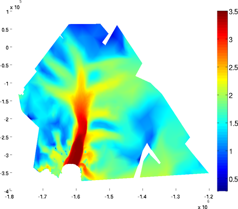
Contours of equi-value can be added to the plot by using the 'contourlevels' option. The number of contours can be chosen by using the 'contourlevels' options. The user can specify a number of levels or a cell containing the values of color changes. For example:
>> plotmodel(md, 'data', md.vel, 'contourlevels', 3)
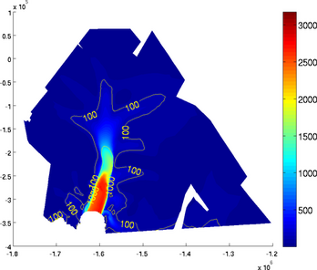
>> plotmodel(md, 'data', md.vel, 'contourlevels', {100, 200, 500, 1000, 2000, 2500})
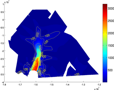
contourticks
If the user does not want to display the contour levels ticks, use the 'contourticks' set as 'off':
>> plotmodel(md, 'data', md.vel, 'contourlevels', {100, 200, 500, 1000, 2000, 2500}, 'contourticks', 'off')
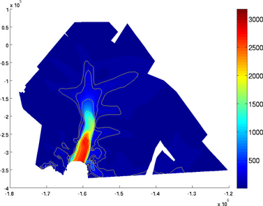
contouronly
If the user wants to display the contours only, use the 'contouronly' set as 'on':
>> plotmodel(md, 'data', 'vel', 'contourlevels', {100, 200, 500, 1000, 2000, 2500}, 'contouronly', 'on')
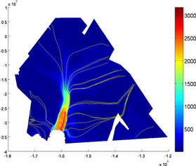
streamlines
Streamlines can be displayed by using the 'streamlines' option followed by a number of streamlines or a cell containing the coordinates of seed points:
>> plotmodel(md, 'data', md.initialization.vel, 'streamlines', 50)
>> plotmodel(md, 'data', md.initialization.vel, 'streamlines', {10^6 * [-1.45 -0.27], 10^6 * [-1.6 0]})

NOTE: Streamlines use the velocities that are in md.initialization. Make sure you transfer the calculated velocities to md.initialization if you want to display the calculated streamlines.
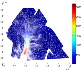
edgecolor
The mesh can be superimposed onto the plot by using the 'edgecolor' option followed by a color:
>> plotmodel(md, 'data', md.initialization.vel, 'edgecolor', 'w')
expdisp
Any ARGUS file can be displayed with the 'expdisp' option followed by the name of the ARGUS file:
>> plotmodel(md, 'data', md.initialization.vel, 'expdisp', 'Iceshelves.exp')
expstyle
The style of the ARGUS profile can be controlled with the 'expstyle' option, followed by the desired line style. Here is an example for a yellow dotted line:
>> plotmodel(md, 'data', md.initialization.vel, 'expdisp', 'Iceshelves.exp', 'expstyle', '--y')
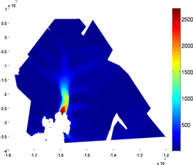
mask
If one does not want to display the value of the field on a mask only, use the 'mask' option followed by a vector that holds 0 for the vertices whose values are hidden:
>> plotmodel(md, 'data', md.initialization.vel, 'mask', md.mask.ocean_levelset < 0)
northarrow
An arrow pointing North can be added with the 'northarrow' option followed by 'on'. The shape and position of the arrow can be controlled by using [x0 y0 length [ratio [width]]] instead of 'on':
>> plotmodel(md, 'data', md.initialization.vel, 'northarrow', 'on')
scaleruler
A scale ruler can be added. As for the North arrow, the default display is done by 'on' but the shape and position of the scale ruler can be controlled by [x0 y0 length width numberofticks] where (x0,y0) are the coordinates of the lower left corner:
>> plotmodel(md, 'data', md.initialization.vel, 'scaleruler', 'on')
title
Same as standard title MATLAB option:
>> plotmodel(md, 'data', md.vel, 'title', 'Ice velocity [m/yr]')
fontsize
Same as standard fontsize MATLAB option:
>> plotmodel(md, 'data', md.vel, 'title', 'Ice velocity [m/yr]', 'fontsize', 8)
fontweight
Same as standard fontweight MATLAB option:
>> plotmodel(md, 'data', md.vel, 'title', 'Ice velocity [m/yr]', 'fontweight', 'b')
xlabel, ylabel
Same as standard xlabel MATLAB option:
>> plotmodel(md, 'data', md.vel, 'xlabel', 'x axis [m]')
Special plots
basaldrag
The special plot 'basal_drag' displays the norm of the basal drag friction in kPa following formula:
Basal drag relies on the velocity provided in md.initialization. The x and y components of the basal drag can be displayed with the 'basal_dragx' or 'basal_dragy' special plots:
>> plotmodel(md, 'data', 'basal_drag')
>> plotmodel(md, 'data', 'basal_dragx')
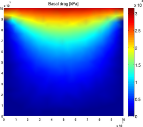
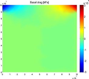
Basal friction norm and Basal friction x-component
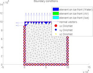
BC
The special plot 'BC' displays all boundary conditions (Newmann and Dirichlet) for 2D and 3D meshes:
>> plotmodel(md, 'data', 'BC')
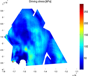
driving_stress
The special plot 'driving_stress' displays the basal drag friction in kPa following formula:
>> plotmodel(md, 'data', 'driving_stress')
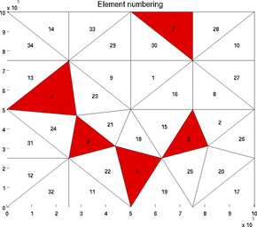
elementnumbering
In the debugging process, it is often very useful to display all the elements next to their numbers. This is what the special plot 'elementnumbering' does:
>> plotmodel(md, 'data', 'elementnumbering')
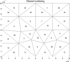
A given list of elements can be highlighted with the 'highlight' option:
>> plotmodel(md, 'data', 'elementnumbering', 'highlight', [3 4 5 6 7])
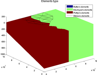
elements_type
The special plot 'elements_type' displays the elements with a specific color for each formulation:
>> plotmodel(md, 'data', 'elements_type')
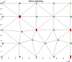
vertexnumbering
In the debugging process, it is often very useful to display all the vertices next to their numbers. This is what the special plot 'vertexnumbering' does:
>> plotmodel(md, 'data', 'vertexnumbering')
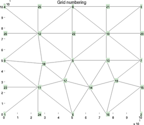
A given list of vertices can be highlighted with the 'highlight' option:
>> plotmodel(md, 'data', 'vertexnumbering', 'highlight', [2 5 7 12])
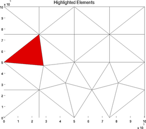
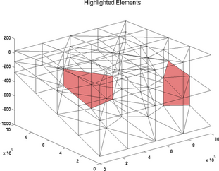
highlightelements
The special plot 'highlightelements' is very similar to the plot 'elementnumbering'. It is another possibility to highlight one or several grids, but without indicating the number of all the elements. It is a lot faster for large models:
>> plotmodel(md, 'data', 'highlightelements', 'highlight', 5)
>> plotmodel(md, 'data', 'highlightelements', 'highlight', [5 12])
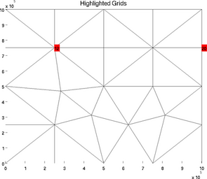
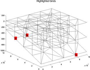
highlightgrids
The special plot 'highlightgrids' is very similar to 'gridnumbering'. It is another possibility to highlight grids without indicating all the grids numbers. It is a lot faster for big models:
>> plotmodel(md, 'data', 'highlightgrids', 'highlight', [12 20])
>> plotmodel(md, 'data', 'highlightgrids', 'highlight', [12 16 26])
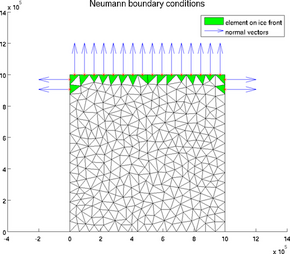
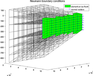
icefront
The special plot 'icefront' displays the Neumann boundary conditions, i.e. all the segments on ice front and the normal to these segments, for a 2D or 3D mesh:
>> plotmodel(md, 'data', 'icefront')
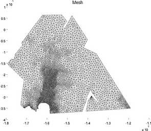
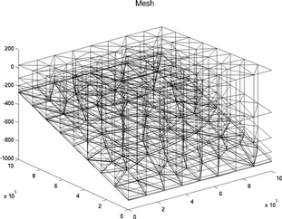
mesh
The special plot 'mesh' displays the mesh of 2D or 3D model:
>> plotmodel(md, 'data', 'mesh')
Quiver plot
For 2D or 3D fields, a generic color plot cannot be used (except component by component). The 'data' used by the function plotmodel must be a matrix of 2 or 3 columns. For example:
>> plotmodel(md, 'data', [md.vx md.vy])

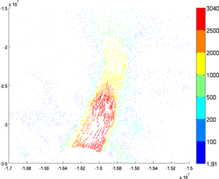
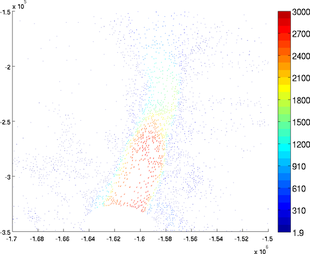
ColorLevels
The number of colors can be chosen by using the 'colorlevels' options. The user can specify a number of levels or a cell containing the values of color changes. For example:
>> plotmodel(md, 'data', [md.vx md.vy], 'colorlevels', 3)
>> plotmodel(md, 'data', [md.vx md.vy], 'colorlevels', 100)
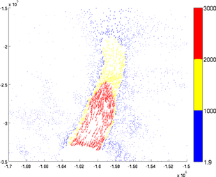
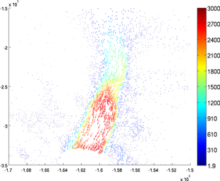
>> plotmodel(md, 'data', [md.vx md.vy], 'colorlevels', {100, 200, 500, 1000, 2000, 2500})
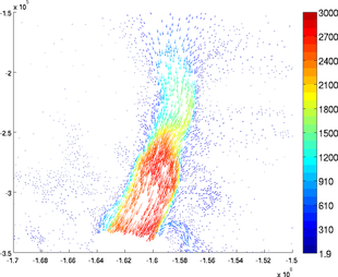
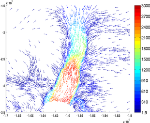
Scaling
The arrows length can be modified with the 'scaling' options. The default value is 0.4. A higher scaling value will result in longer arrows:
>> plotmodel(md, 'data', [md.vx md.vy], 'scaling', 1)
>> plotmodel(md, 'data', [md.vx md.vy], 'scaling', 0.1)
Autoscale
If the user wants all the arrows to have the same length, use the option 'autoscale' set as 'off':
>> plotmodel(md, 'data', [md.vx md.vy], 'autoscale', 'off')
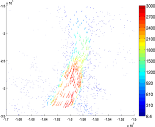
Density
The number of arrows can be reduced with the option 'density'. If the density is set as 3, only one arrow out of 3 will be displayed. This option is very useful when the mesh is very refined:
>> plotmodel(md, 'data', [md.vx md.vy], 'density', 3)
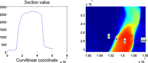
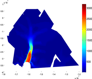
Cross section
The section plot can be used to display the value of a field on a given track. The option 'sectionvalue' must be followed by the name of an ARGUS file which contained the coordinates of the points describing the profile (this file can be generated by exptool.m). The resulting plot will be a curve in 2D and a colored surface in 3D. For example:
>> plotmodel(md, 'data', md.vel, 'expdisp', 'track.exp')
>> plotmodel(md, 'data', md.vel, 'sectionvalue', 'track.exp')
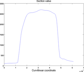
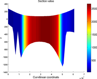
Section plot for 2D (left) and 3D (right) models
Resolution
The horizontal and vertical (in 3D) resolution can be specified by the 'resolution' option. It must be a list with the horizontal resolution followed by the vertical resolution (in meters). When not specified, the default resolution is displayed:
>> plotmodel(md, 'data', md.vel, 'sectionvalue', 'track.exp', 'resolution', [2*10^4 0])
>> plotmodel(md, 'data', md.vel, 'sectionvalue', 'track.exp', 'resolution', [10^3 0])
Show section
The profile used to create the section plot can be also plotted with the 'showsection' option:
>> plotmodel(md, 'data', md.vel, 'showsection', 'on')