Modeling Helheim Glacier

Goals

Create an ice-flow model of Helheim Glacier (southeast Greenland)
Run an inversion model to infer basal friction

Introduction

In this example, the main goal is to parameterize and model a real Greenland outlet glacier. In order to build an operational simulation of Helheim Glacier, we will follow these steps:

Define the model region
Create a mesh
Parameterize the model
Invert for friction coefficient
Plot results

Files needed for this tutorial can be found in <ISSM_DIR>/examples/Helheim/. The runme.m file contains the structure of the simulation, while the .par file includes most parameters needed for the model set-up. The .exp file contains coordinates that define the model domain boundaries.

Observed datasets needed for the parameterization need to be downloaded.

Mesh

The first step is to create the model domain outline and mesh.

In the runme.m file, the mesh is generated in a multi-step process. Open the runme.m file and make sure that the variable steps, at the top of the file, is set to steps = [1]. In the code, you will see that in Step 1 the following actions are implemented:

Create a uniform mesh
Refine the mesh using anisotropic mesh refinement based on surface velocity
Set the mesh parameters
Load observed surface velocities
Interpolate velocity onto a coarse mesh. Adapt the mesh to minimize error in velocity interpolation
Save the model

Execute the runme.m file to perform step 1. Plot the mesh with:

plotmodel(md, 'data', 'mesh')

You should see the following figure, with finer resolution in the two main branches of Helheim and its main trunk:

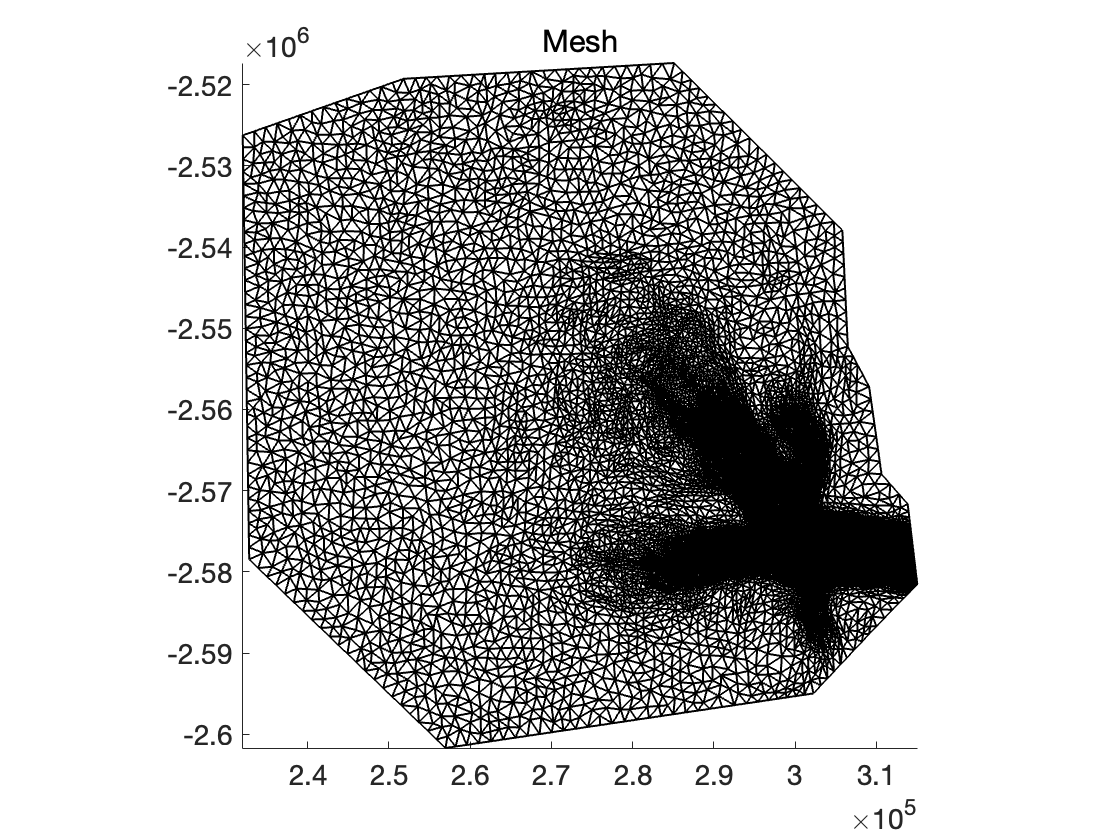
Try experimenting with different values in the mesh generation to create finer or coarser meshes.

Parameterization

Most of the model parameterization is done through a different file (Greenland.par). In this example, we parameterize the following model fields:

Geometry (ice surface elevation and bed topography, using BedMachine)
Initialization parameters
Material parameters
Friction coefficient
Boundary conditions

Run step 2 in the runme.m file to perform the parameterization.

Inversion for basal friction

The friction coefficient is inferred from the surface velocity using the following friction law:

$Equation 1$

$Equation 2$ : Basal stress (basal drag)
$Equation 3$ : Effective pressure (ice overburden pressure - water pressure at the bed)
$Equation 4$ : Basal velocity (equal to surface velocity in SSA approximation)
$Equation 6$ : Exponent (equals $Equation 5$ of the parameter file)
$Equation 8$ : Exponent (equals $Equation 7$ of the parameter file)

The procedure for the inversion is as follows:

Velocity is computed from the SSA approximation
Misfit of the cost function is computed
Friction coefficient is modified following the gradient of the cost function

All the parameters that can be adjusted for the inversion are in md.inversion.

Run step 3. This will take a few minutes to run. Plot the resulting velocity and friction coefficient:

plotmodel(md, 'data', md.initialization.vel, 'title', 'Surface Velocity (m/yr)', ...
	'data', md.friction.coefficient, 'title', 'Friction Coefficient')

You should see something similar to the figure below:

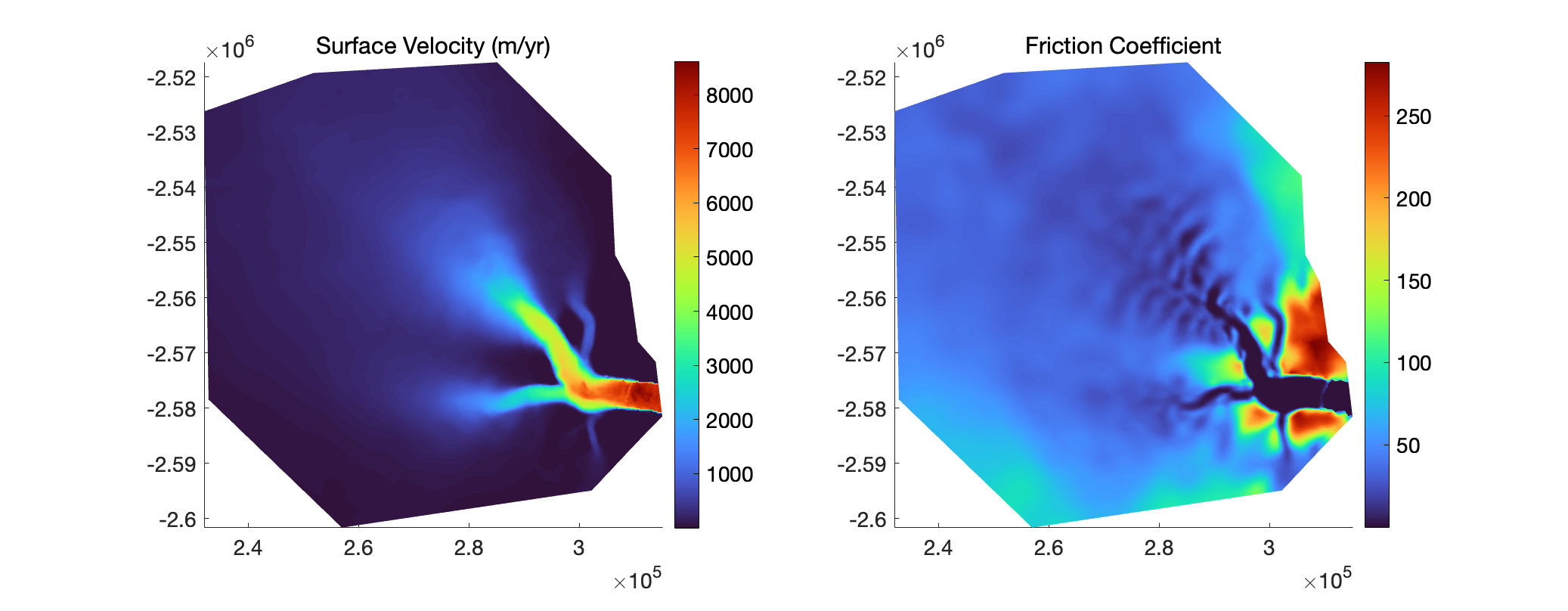
Try experimenting with different cost-function values and other parameters in md.inversion.

Now that you have run an inversion for basal friction and have a working stress-balance model of Helheim Glacier, you are ready for the next tutorial on simulating subglacial hydrology at Helheim using the SHAKTI model.