Pine Island Glacier Stochastic Forcing (StISSM)
Goals
- Introduction to the use of the stochastic capabilities implemented in ISSM (StISSM)
- Model Pine Island Glacier as in previous tutorials, but with stochastic forcings
Introduction
The main goals of this tutorial are 1) to become familiar with the use of StISSM, 2) to learn how to parameterize stochastic variables of the model, and 3) to launch transient stochastic simulations. The first steps follow what was done in previous tutorials: setting up the model domain and general configuration for the Pine Island Glacier. The organization of the tutorial is as follows:
- Step 1: Generate a model mesh
- Step 2: Set up the ice and ocean masks
- Step 3: Parameterization of the model
- Step 4: Set up the stochastic SMB parameterization
- Step 5: Transient run
- Step 6: Set up the stochastic calving parameterization
- Step 7: Second transient run starting from the results of the first one Files needed for this tutorial can be found in
trunk/examples/StISSM/. Therunme.mfile contains the structure of the overall simulation, while the .par file includes most parameters needed for the model setup. The.expfiles are domain files that define geometric boundaries of the simulation. Observed datasets needed for the parameterization also need to be downloaded.
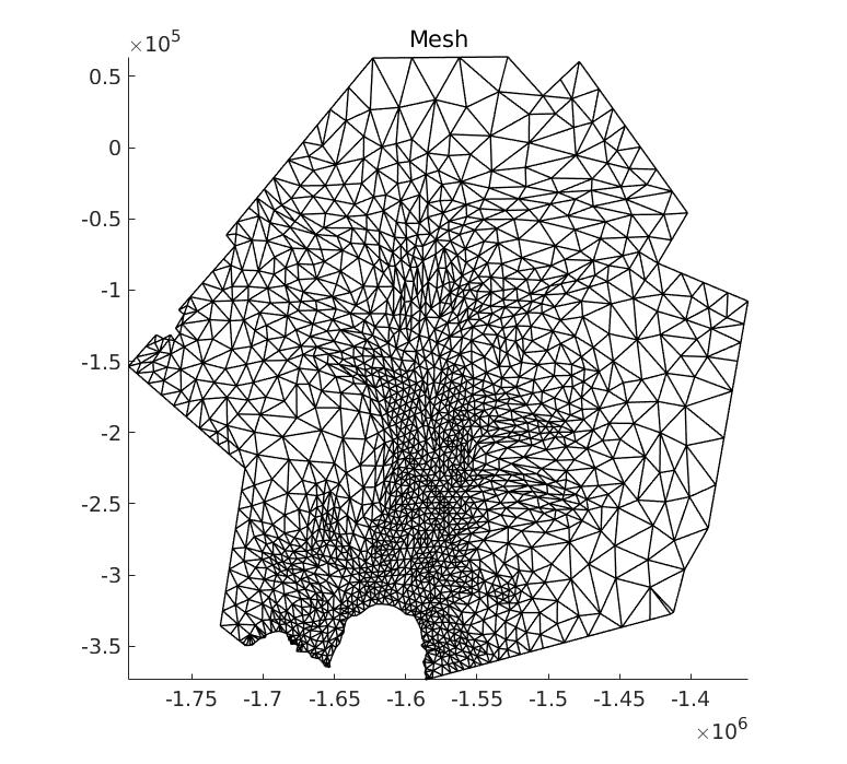
Mesh
This step follows what is done in the Pine Island Glacier tutorial. We simply set up the model mesh from the exp files. Set step = 1 in the runme.m file to execute it.
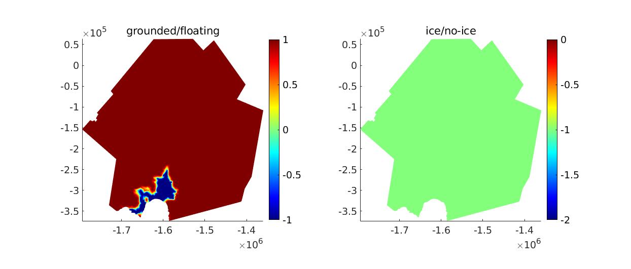
Mask
This step follows what is done in the Pine Island Glacier tutorial. We define the masks where ice is present/absent and where ice is grounded/floating. Set step = 2 in the runme.m file to execute it.
Parameterization
This step follows what is done in the Pine Island Glacier tutorial. We use the PigStISSM.par file to parameterize the following fields:
- Geometry
- Initialization parameters
- Material parameters
- Forcings
- Friction coefficient
- Ice rheology
- Boundary conditions Set
step = 3in therunme.mfile to execute it.
Parameterization
From here, we start to focus on the specifics of StISSM. We set up an Autoregressive Moving-Average (ARMA) model for SMB. In other words, the evolution of SMB follows the following equation:
where is a deterministic function of time,
are the autoregressive (AR) coefficients, and
are the moving-average coefficients (MA). The values of
and
are the orders of the AR and MA part of the ARMA model, respectively. The term
is a Gaussian noise term generated at time step
.
We define two different subdomains, with separate ARMA processes. The subdomains are separated at 1/3rd of the x-axis. For the deterministic function in Eq. (1), we use a piecewise linear function with a single breakpoint:
where is the initial time of the ARMA model,
is the breakpoint (a date in time), the
terms are constant values, and the
terms are trends in time. All the coefficients and parameters of Eqs (1) and (2) are prescribed in the runme.m file.
Next, we also define some SMB lapse rates. Lapse rates are elevation gradient of SMB. The lapse rate values must be associated with an elevation range, such that lapse rate 1 applies below elevation 1, lapse rate 2 applies between elevation 1 and elevation 2, etc.
After that, we set up the covariance matrix that will define the stochastic perturbations. We use different amplitudes of variability in the two subdomains, and a moderate correlation (0.5) between the subdomains. Notice that the covariance matrix is simply computed as:
where is the diagonal matrix with the individual standard deviations on the diagonal, and
is the correlation matrix.
The final step of the stochasticity configuration is to set up the parameterization of md.stochasticforcing. This only entails activating stochasticity, specifying which model field is stochastic (SMBarma here), the time step of stochasticity (the frequency at which random perturbations are generated), and assigning the covariance matrix. Set step = 4 in the runme.m file to execute this step.
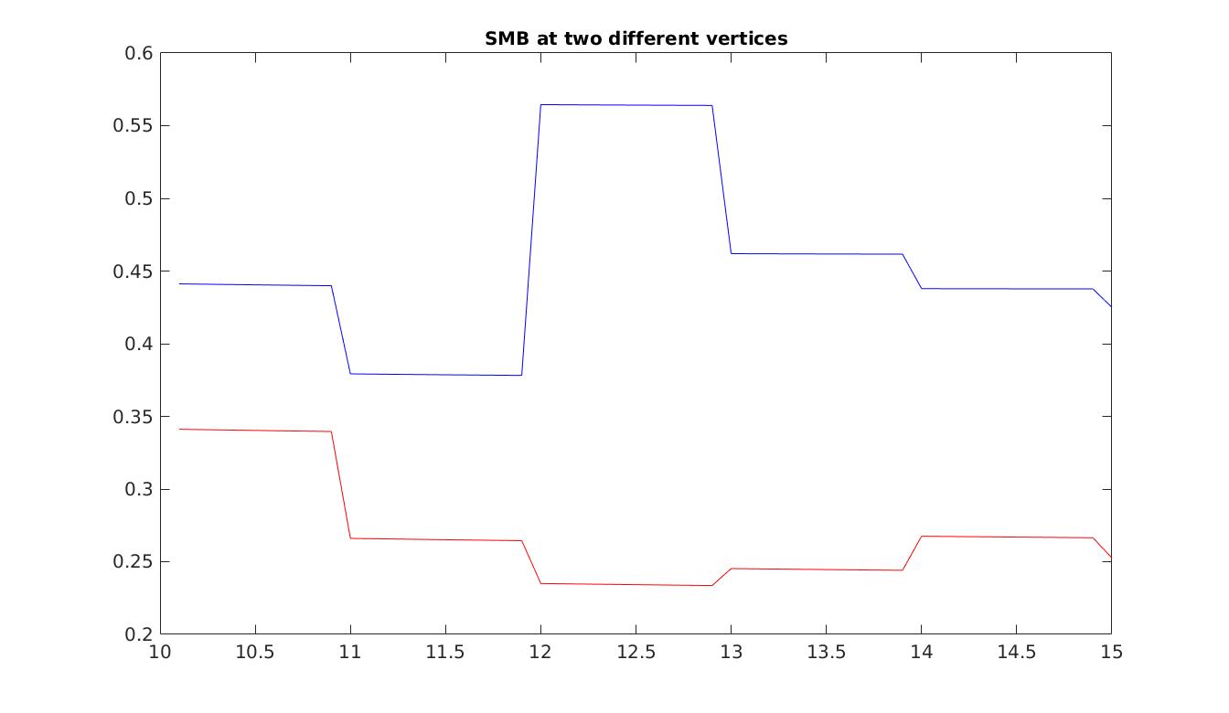
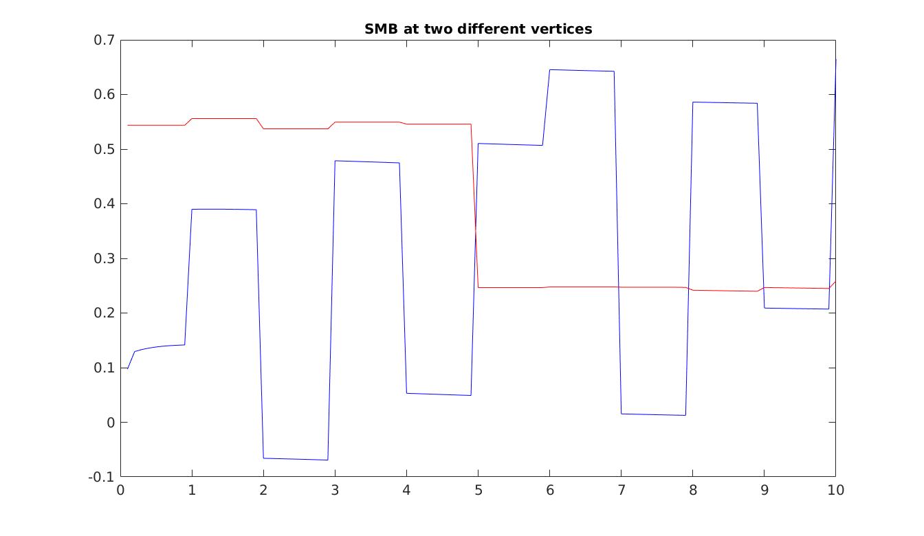
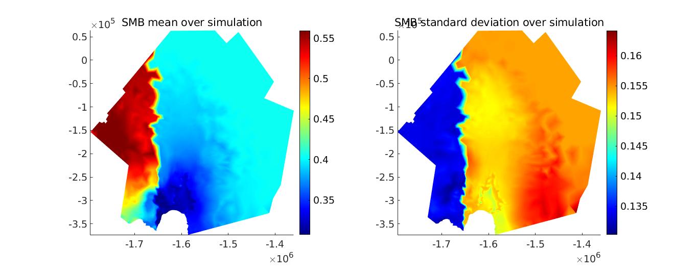
Transient run 1
Now that the entire model is configured, we run a transient simulation and plot some results. The plots generated are an example of the SMB results that you could reach. Note that all runs will have different SMB fields, due to stochasticity. Set step = 5 in the runme.m file to execute it.
Stochastic calving
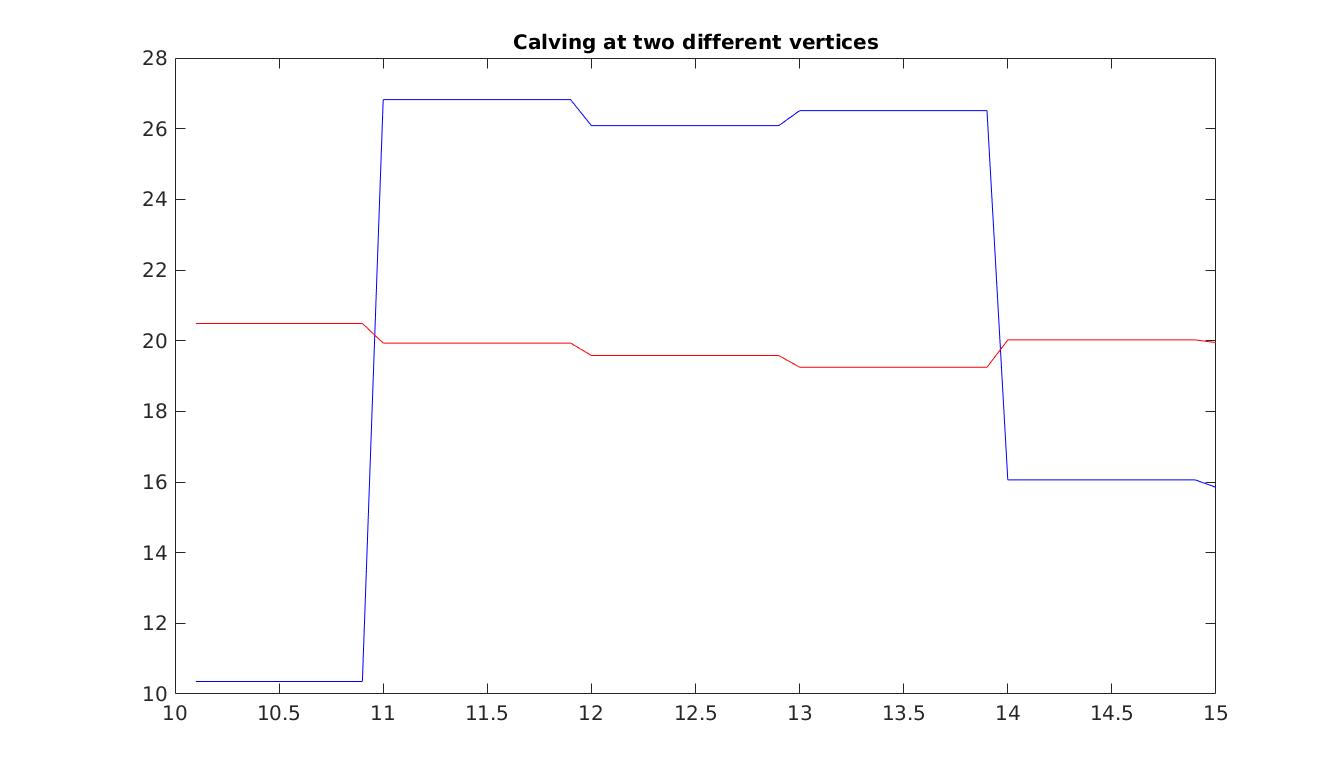
In the last step of this tutorial, we also want to activate stochastic calving. First, we need to specify that calving at the ice front is activated, and specify the background calving values. Notice also that imposing calving means that we need to allow for the ice front to migrate by setting md.transient.ismovingfront to 1. Here, we assign the same subdimensions for calving as for SMB. Next, we need to set the covariance matrix for calving. This involves setting the individual standard deviations for the two subdomains, the correlation matrix (here, we set no correlation), and applying Eq. (3). Finally, we modify the md.stochasticforcing class. We specify that two fields are stochastic [{SMBarma’}, {DefaultCalving'}]. We stack the SMB and calving covariance matrices together, here assuming no correlation between these different fields. As a final note, calving is not an ARMA model, thus its subdimensions must be passed as the default dimensions of the md.stochasticforcing class. Set step = 6 in the runme.m file to execute this step.
Transient run 2
We want to launch a second transient run. First, we load the final geometry, masks, and velocities of the previous transient run, and set these as initial conditions for the second transient run. The model is now fully configured for the second transient run. We launch the transient simulation, and plot some results. Again, the plots generated are an example of possible results, which will vary due to the stochastic nature of the model run. Set step = 7 in the runme.m file to execute this step.